Calling structures from single cells

One single-cell Hi-C map holds 10⁴–10⁶ contacts, too few for the callers of bulk Hi-C. This tutorial goes through the four routes U-Chrom offers instead, on real data, each checked against an independent reference:

1. loops across cells without pooling them — SnapHiC: every cell’s map imputed by a random walk with restart, every candidate pixel tested against its local background over the cells;

2. domain boundaries of single cells — the insulation of each cell’s imputed map, and their consensus;

3. compartment values of every cell — scA/B, the mean CpG frequency of each bin’s contact partners;

4. the tracing callers on reconstructed 3-D structures — a reconstruction is a ChromData with coordinates.

• Data: Nagano et al. 2017 diploid mES cells (ds.load("nagano2017_dip_serum"): 1,175 cells, 10 kb maps per cell; the 742 deepest, as SnapHiC used), with SnapHiC’s published loops and reference lists (yu2021_snaphic) and the bulk Hi-C of Bonev et al. 2017 (bonev2017_mesc_4dn); Tan et al. 2018 Dip-C GM12878 structures (ds.load("tan2018_gm12878")) against Rao et al. 2014 GM12878 Hi-C.

• Runtime: about 20 min on 32 cores with the native kernels (uchrom-maps); this notebook was executed on a cluster node (Sherlock).

import os
import time
from pathlib import Path

import matplotlib.pyplot as plt
import numpy as np
import pandas as pd

import uchrom as uc
import uchrom.datasets as ds
from uchrom.fea import add_sequence_features, contact_matrix, rebin_map
from uchrom.io import read_juicer_loops
from uchrom.strc.comp import CompartmentCallerParams, compare_compartments
from uchrom.strc.loop import match_loops
from uchrom.strc.tad import compare_boundaries

plt.rcParams["figure.dpi"] = 90
OUT = Path("_out") / "sc_structures"; OUT.mkdir(parents=True, exist_ok=True)   # outputs: tutorials/_out/
THREADS = int(os.environ.get("SLURM_CPUS_PER_TASK", os.cpu_count()))
T0 = time.time()

cd = ds.load("nagano2017_dip_serum", backed=True)        # built once from the original files (fetch + loader)
top = cd.cells.index[cd.cells["snaphic_top742"]]        # SnapHiC's cells: the 742 with the most contacts
print(cd)
cd.cells.loc[top].groupby("group", observed=True).agg(cells=("n_contacts", "size"),
                                                      median_contacts=("n_contacts", "median"))

ChromData (backed: nagano2017_dip_serum.chromdata.zarr): n_spots=0, n_traces=0, n_cells=1175, n_bins=0
  spots:   ['chrom', 'start', 'end', 'trace_id', 'cell_id', 'bin_id']
  cells:   ['batch_name', 'cond', 'group', 'passed_qc', 'total_contacts', 'f_trans', 'repli_score', 'n_fend_pairs', 'n_unmapped', 'n_contacts', 'n_cis', 'n_trans', 'frac_cis', 'snaphic_top742', 'cell_type'] (1175 cells)
  uns:     ['genome_assembly', 'source', 'haplotypes', 'linked_scool', 'dataset']

	cells	median_contacts
group
G1	128	293240.0
early-S	302	310313.5
late-S/G2	265	317862.0
post-M	4	354351.0
pre-M	14	360648.0

1. Loops across cells: SnapHiC

uc.tl.call_loops(cd, method="snaphic") imputes each cell’s map (whole chromosomes, 10 kb), turns it into per-diagonal z-scores and tests every pixel against its local background over the cells (paired t-test, FDR per distance, SnapHiC’s filters and clustering). It excludes SnapHiC’s low-mappability bins. Two chromosomes here, to keep the notebook short (genome-wide: ~1.5 h on 32 cores).

CHROMS = ["chr18", "chr19"]
exclude = ds.fetch("snaphic_filter_regions", verbose=False) / "mm10_filter_regions.txt"
t = time.time()
loops = uc.tl.call_loops(cd, method="snaphic", cells=top, chrom=CHROMS, exclude=exclude, n_threads=THREADS)
print(f"{len(loops):,} loops on {', '.join(CHROMS)} from {len(top)} cells in {time.time() - t:.0f} s")
loops.head(3)

1,353 loops on chr18, chr19 from 742 cells in 229 s

	chrom1	start1	end1	chrom2	start2	end2	score	outlier_count	pvalue	tstat	fdr_dist	case_avg	control_avg	circle	donut	horizontal	vertical	lower_left	cluster_size	neg_log10_fdr
0	chr18	3260000	3270000	chr18	4000000	4010000	3.173759	122	2.968312e-05	4.202004	0.000670	0.908661	0.515784	74.906250	75.317460	87.666667	87.500000	66.428571	108	556.775533
1	chr18	3260000	3270000	chr18	4150000	4160000	2.501121	128	1.982755e-04	3.739928	0.003154	1.066955	0.665968	87.552083	87.460317	95.166667	103.833333	81.000000	108	556.775533
2	chr18	3270000	3280000	chr18	3420000	3430000	5.676689	123	1.636099e-07	5.287178	0.000002	0.701035	0.329022	73.302083	68.047619	86.666667	86.833333	81.380952	108	556.775533

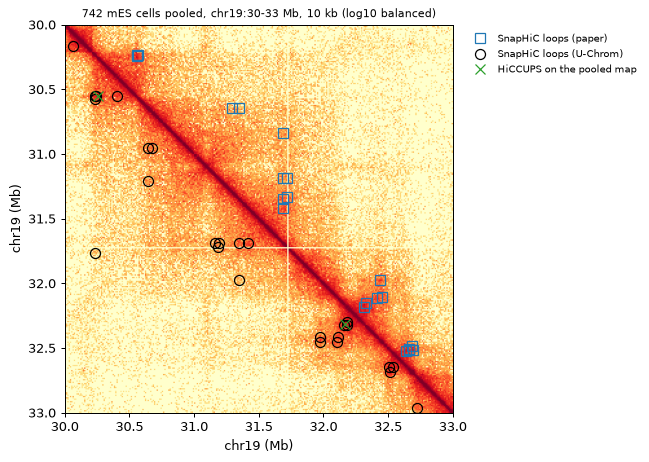
The paper’s measures (Yu et al. 2021): a call overlaps a loop when both anchors are within 20 kb; precision against the combined mESC reference (HiCCUPS on bulk Hi-C + MAPS on H3K4me3 PLAC-seq, cohesin and H3K27ac HiChIP), recall of the bulk HiCCUPS loops, both in 100 kb – 1 Mb. The paper’s own calls from the same 742 cells are the yardstick.

src = ds.fetch("yu2021_snaphic", verbose=False)         # the paper's source data (two workbooks)
refs = src / "41592_2021_1231_MOESM6_ESM.xlsx"
def in_range(t):                                     # loops of CHROMS, anchors 100 kb - 1 Mb apart
    sep = t["start2"] - t["start1"]
    return t[t["chrom1"].isin(CHROMS) & (sep >= 100_000) & (sep <= 1_000_000)].reset_index(drop=True)

bulk_hiccups = in_range(read_juicer_loops(refs, sheet="Bulk_HiC_filter"))
reference = in_range(pd.concat([read_juicer_loops(refs, sheet=f"{s}_filter") for s in
                                ("Bulk_HiC", "H3K4me3_PLACseq", "cohesin_HiChIP", "H3K27ac_HiChIP")])
                     .drop_duplicates(["chrom1", "start1", "start2"]))
paper = in_range(read_juicer_loops(src / "41592_2021_1231_MOESM4_ESM.xlsx", sheet="Permu0_742"))

def scores(calls):
    calls = in_range(calls)
    return {"loops": len(calls), "precision": match_loops(calls, reference, tol=20_000).mean(),
            "recall": match_loops(bulk_hiccups, calls, tol=20_000).mean()}

rows = {"U-Chrom SnapHiC": scores(loops), "the paper's SnapHiC": scores(paper)}
print(f"{len(paper)} paper loops; {match_loops(paper, loops, tol=20_000).mean():.0%} of them within 20 kb of ours")
pd.DataFrame(rows).T.round(2)

1090 paper loops; 76% of them within 20 kb of ours

	loops	precision	recall
U-Chrom SnapHiC	1292.0	0.62	0.61
the paper's SnapHiC	1090.0	0.67	0.60

What pooling the same cells gives instead: their maps summed into one pseudo-bulk map, then HiCCUPS — and the pileup of SnapHiC’s loops on that map (APA, with the loops shifted by ±0.5 / ±1 Mb as the control).

t = time.time()
uc.tl.pseudobulk(cd, pd.Series("top742", index=top), trans=False, key_prefix="pooled", out_dir=OUT)
pooled = uc.tl.call_loops(cd, method="hiccups", contacts="pooled.top742", chrom=CHROMS, key_added="loops.pooled")
apa = uc.tl.pileup(cd, loops, contacts="pooled.top742", shifts=(-1_000_000, -500_000, 500_000, 1_000_000),
                   key_added=None)
rows["HiCCUPS on the pooled map"] = scores(pooled)
print(f"pooled map + HiCCUPS in {time.time() - t:.0f} s; APA of the SnapHiC loops on it {apa['apa']:.2f} "
      f"(shifted {apa['control']:.2f})")
pd.DataFrame(rows).T.round(2)

pooled map + HiCCUPS in 2 s; APA of the SnapHiC loops on it 1.93 (shifted 0.98)

	loops	precision	recall
U-Chrom SnapHiC	1292.0	0.62	0.61
the paper's SnapHiC	1090.0	0.67	0.60
HiCCUPS on the pooled map	34.0	0.97	0.06

R0, R1, RES = 30_000_000, 33_000_000, 10_000
bins, M = contact_matrix(cd, "pooled.top742", chrom="chr19")
lo, hi = R0 // RES, R1 // RES
x0, x1 = R0 / 1e6, R1 / 1e6
def mids(t):
    t = t[(t["chrom1"] == "chr19") & (t["start1"] >= R0) & (t["end2"] <= R1)]
    return (t["start1"] + t["end1"]) / 2e6, (t["start2"] + t["end2"]) / 2e6

fig, ax = plt.subplots(figsize=(6, 5.6))
ax.imshow(np.log10(M[lo:hi, lo:hi] + 1e-6), cmap="YlOrRd", vmin=-3.6, vmax=-1.2, extent=[x0, x1, x1, x0])
a, b = mids(paper);  ax.plot(b, a, "s", mfc="none", mec="C0", ms=8, label="SnapHiC loops (paper)")
a, b = mids(loops);  ax.plot(a, b, "o", mfc="none", mec="k", ms=8, label="SnapHiC loops (U-Chrom)")
a, b = mids(pooled); ax.plot(a, b, "x", color="C2", ms=8, label="HiCCUPS on the pooled map")
ax.set_xlim(x0, x1); ax.set_ylim(x1, x0); ax.set_xlabel("chr19 (Mb)"); ax.set_ylabel("chr19 (Mb)")
ax.set_title(f"742 mES cells pooled, chr19:{x0:.0f}-{x1:.0f} Mb, 10 kb (log10 balanced)", fontsize=9)
ax.legend(loc="upper left", bbox_to_anchor=(1.02, 1), fontsize=8, frameon=False)
plt.show()

2. Domain boundaries of single cells

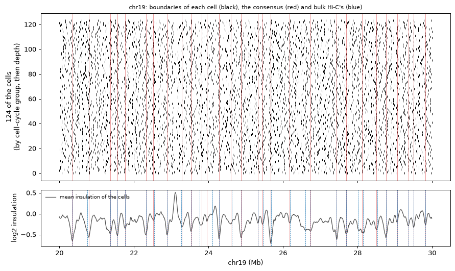
uc.tl.single_cell_boundaries computes the insulation score of each cell’s imputed map, each cell’s boundaries, and consensus boundaries from the cells’ mean insulation. The reference is the insulation of bulk Hi-C of the same cell type (Bonev et al. 2017, 10 kb, 100 kb window).

t = time.time()
sc_bounds = uc.tl.single_cell_boundaries(cd, cells=top, chrom="chr19", per_cell=True, n_threads=THREADS)
print(f"chr19, {len(top)} cells in {time.time() - t:.0f} s: {int(sc_bounds['consensus'].sum())} consensus boundaries")

cd.link_cool(ds.path("bonev2017_mesc_4dn"), key="bonev")              # bulk mESC Hi-C (4DN mcool)
uc.tl.call_tads(cd, method="insulation", contacts="bonev", resolution=10_000, chrom="chr19", key_added="tads.bonev")
consensus = pd.DataFrame(cd.intervals["tads.single_cell.domains"])
near = compare_boundaries(cd, consensus, "tads.bonev", tol=2, contacts="bonev", resolution=10_000)
found = compare_boundaries(cd, "tads.bonev", consensus, tol=2, contacts="bonev", resolution=10_000)
print(f"consensus boundaries near a bulk boundary (±2 bins): {near['fraction_near']:.2f} (chance {near['chance']:.2f}); "
      f"bulk boundaries recovered: {found['fraction_near']:.2f} (chance {found['chance']:.2f})")
bulk_ins = cd.results["tads.bonev.score"]
both = sc_bounds.merge(bulk_ins[["chrom", "start", "log2_insulation_score_100000"]], on=["chrom", "start"])
print("mean single-cell insulation vs bulk insulation, Spearman "
      f"{both['insulation'].corr(both['log2_insulation_score_100000'], method='spearman'):.2f}")

chr19, 742 cells in 45 s: 179 consensus boundaries

consensus boundaries near a bulk boundary (±2 bins): 0.73 (chance 0.14); bulk boundaries recovered: 0.76 (chance 0.15)
mean single-cell insulation vs bulk insulation, Spearman 0.65

R0, R1 = 20_000_000, 30_000_000
per_cell = cd.results["tads.single_cell.cells"]
view = sc_bounds[(sc_bounds["start"] >= R0) & (sc_bounds["start"] < R1)]
order = cd.cells.loc[top].sort_values(["group", "n_contacts"]).index[::6]   # every 6th cell, for legibility
row = {c: k for k, c in enumerate(order)}
pc = per_cell[(per_cell["start"] >= R0) & (per_cell["start"] < R1) & per_cell["cell_id"].isin(row)]
bulk_b = cd.results["tads.bonev.boundaries"]
bulk_b = bulk_b[(bulk_b["chrom"] == "chr19") & (bulk_b["start"] >= R0) & (bulk_b["start"] < R1)]

fig, (a1, a2) = plt.subplots(2, 1, figsize=(10, 6), sharex=True, gridspec_kw={"height_ratios": [3, 1]})
a1.scatter(pc["start"] / 1e6, [row[c] for c in pc["cell_id"]], s=14, c="k", marker="|", lw=0.8)
a1.set_ylabel(f"{len(order)} of the cells\n(by cell-cycle group, then depth)")
a1.set_title("chr19: boundaries of each cell (black), the consensus (red) and bulk Hi-C's (blue)", fontsize=9)
a2.plot(view["start"] / 1e6, view["insulation"], color="0.3", lw=1, label="mean insulation of the cells")
for s in view.loc[view["consensus"], "start"] / 1e6:
    a1.axvline(s, color="C3", lw=0.6, alpha=0.6); a2.axvline(s, color="C3", lw=0.6, alpha=0.6)
for s in bulk_b["start"] / 1e6:
    a2.axvline(s, color="C0", lw=0.6, ls="--")
a2.set_xlabel("chr19 (Mb)"); a2.set_ylabel("log2 insulation"); a2.legend(fontsize=8, frameon=False)
plt.tight_layout(); plt.show()

3. Compartment values of every cell: scA/B

uc.tl.single_cell_compartments gives each cell and bin the mean CpG frequency of the bin’s contact partners in that cell (Tan et al. 2021, Dip-C), ranked per cell. Against the compartment eigenvector (E1) of the pooled map of the same cells:

genome = ds.fetch("mm10_genome", verbose=False)       # UCSC mm10: CpG (scA/B) and GC (E1 phasing) per bin
AUTOSOMES = [f"chr{k}" for k in range(1, 20)]
t = time.time()
scab = uc.tl.single_cell_compartments(cd, cells=top, track=genome, resolution=1_000_000, chrom=AUTOSOMES)
print(f"scA/B: {scab.shape[0]} cells x {scab.shape[1]} bins in {time.time() - t:.0f} s")

rebin_map(cd, "pooled.top742", resolution=1_000_000, key_added="pooled_1mb")
e1 = uc.tl.call_compartments(cd, method="eig", contacts="pooled_1mb", chrom=AUTOSOMES, phasing=genome)
e1.index = e1["chrom"].astype(str) + ":" + e1["start"].astype(str) + "-" + e1["end"].astype(str)
common = scab.columns.intersection(e1.index)
r = scab[common].T.corrwith(e1.loc[common, "E1"])         # each cell's scA/B vs the pooled E1
cellr = cd.cells.loc[r.index].assign(r=r.values)
print(f"mean scA/B vs pooled E1: r = {np.corrcoef(scab[common].mean(), e1.loc[common, 'E1'])[0, 1]:.2f}; "
      f"per cell: median r = {r.median():.2f}")
cellr.groupby("group", observed=True)["r"].agg(["size", "median"]).round(2)

scA/B: 742 cells x 2473 bins in 95 s

mean scA/B vs pooled E1: r = 0.80; per cell: median r = 0.75

	size	median
group
G1	128	0.67
early-S	302	0.76
late-S/G2	265	0.75
post-M	4	0.51
pre-M	14	0.69

chr_ = "chr2"
cols = [c for c in common if c.startswith(chr_ + ":")]
order = cellr.sort_values(["group", "n_contacts"]).index
fig = plt.figure(figsize=(11, 4.6))
gs = fig.add_gridspec(2, 2, height_ratios=[1, 5], width_ratios=[3, 1.3], hspace=0.05, wspace=0.3)
axe = fig.add_subplot(gs[0, 0]); axh = fig.add_subplot(gs[1, 0], sharex=axe); axs = fig.add_subplot(gs[:, 1])
x = np.arange(len(cols)); v = e1.loc[cols, "E1"].to_numpy()
axe.bar(x, v, width=1, color=np.where(v > 0, "C3", "C0")); axe.set_ylabel("E1"); axe.tick_params(labelbottom=False)
axe.set_title(f"{chr_} at 1 Mb: pooled E1 (top) and every cell's scA/B (rows, by cell-cycle group)", fontsize=9)
axh.imshow(scab.loc[order, cols].to_numpy(), aspect="auto", cmap="RdBu_r", interpolation="none")
axh.set_xlabel(f"{chr_} (Mb)"); axh.set_ylabel("cells")
for k, (g, sub) in enumerate(cellr.groupby("group", observed=True)):
    axs.scatter(sub["n_contacts"] / 1e3, sub["r"], s=6, label=g, color=f"C{k}")
axs.set_xscale("log"); axs.set_xlabel("contacts per cell (thousands)"); axs.set_ylabel("r with the pooled E1")
axs.xaxis.set_major_formatter(plt.FuncFormatter(lambda v, _: f"{v:g}")); axs.xaxis.set_minor_formatter(plt.NullFormatter())
axs.legend(fontsize=7, frameon=False)
plt.show()

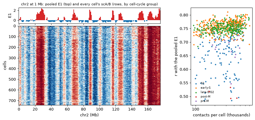
G1 cells follow the pooled E1 less than the cells in S and G2 at the same depth (median r 0.67 against 0.75 in the table above) — the per-cell values carry the cell’s state, not only its depth. Much of scA/B is the CpG track itself (CpG-rich bins contact CpG-rich bins): the cell-type-specific part is smaller than the correlation suggests (see calling structures from single cells), and cells with few contacts are noisy.

4. The tracing callers on reconstructed structures

ds.load("tan2018_gm12878") holds the authors’ Dip-C structures of 14 GM12878 cells (20 kb particles, one trace per cell, chromosome and homolog) next to their per-cell maps. The tracing callers take it as they take imaging; the reference is the E1 of bulk Hi-C (Rao et al. 2014), and the pooled maps of the same cells.

gm = ds.load("tan2018_gm12878", backed=True)
print(gm)
chr21 = gm.get_chrom("chr21")                                  # in memory: 28 homolog traces, 20 kb particles
hg19_chr21 = ds.fetch("hg19_chr21", verbose=False)
add_sequence_features(chr21, ds.fetch("hg19_genome", verbose=False), features=["gc_fraction"])   # GC per locus
                                                               # (every bin of the genome): names A (GC-rich), as E1
t = time.time()
struct = uc.tl.call_compartments(chr21, method="axes_pc", params=CompartmentCallerParams(a_track="seq.gc_fraction"),
                                 key_added=None)               # from the 3-D distances
print(f"compartments from {chr21.n_traces} chr21 structures in {time.time() - t:.0f} s")

gm.link_cool(ds.fetch("rao2014_gm12878_chr21", verbose=False), key="rao")
rebin_map(gm, "rao", resolution=100_000, key_added="rao_100kb")
rao = uc.tl.call_compartments(gm, method="eig", contacts="rao_100kb", chrom="chr21",
                              phasing=hg19_chr21, key_added="compartments.rao")
uc.tl.pseudobulk(gm, trans=False, key_prefix="pooled", out_dir=OUT)            # the same 14 cells' contacts
rebin_map(gm, "pooled.all", resolution=100_000, key_added="pooled_100kb")
pooled_e1 = uc.tl.call_compartments(gm, method="eig", contacts="pooled_100kb", chrom="chr21",
                                    phasing=hg19_chr21, key_added=None)
pd.DataFrame({"structures (axes PC)": compare_compartments(chr21, struct, rao),
              "pooled map (E1)": compare_compartments(chr21, pooled_e1, rao)}).T[["agreement", "pearson_r"]].round(2)

ChromData (backed: tan2018_gm12878.chromdata.zarr): n_spots=3832898, n_traces=639, n_cells=14, n_bins=140938
  spots:   ['chrom', 'start', 'end', 'trace_id', 'cell_id', 'bin_id']
  cells:   ['gsm', 'cell_type', 'dataset', 'n_lines', 'n_contacts', 'n_cis', 'n_trans', 'n_dropped', 'n_pixels_5kb', 'frac_cis', 'n_particles', 'n_traces', 'rmsd_rep1', 'median_dev_rep1', 'rmsd_rep2', 'median_dev_rep2'] (14 cells)
  spot_tracks:    ['rep_deviation']
  traces:  ['cell_id', 'chrom', 'homolog', 'n_particles'] (639 traces)
  layers:  ['rep1', 'rep2']
  uns:     ['genome_assembly', 'source', 'haplotypes', 'linked_scool', 'structures', 'xyz_unit', 'dataset']

compartments from 28 chr21 structures in 144 s

	agreement	pearson_r
structures (axes PC)	0.86	0.76
pooled map (E1)	0.95	0.94

Compartments come out of the structures (and, on 28 homologs, about as well as from imaging with as many traces); the tracing callers do not find TADs or loops on tens of reconstructions — pool the cells or call across them (routes 1 and 2) for those.

Structure	Route that works with tens to hundreds of cells
loops	across cells (SnapHiC), ≥ ~100 cells of a type; pooled maps only at near-bulk depth
domain boundaries	across cells (consensus of single-cell boundaries) or a pooled map
compartments	per cell (scA/B), pooled maps, or reconstructed structures

print(f"total run time {(time.time() - T0) / 60:.1f} min")

total run time 11.4 min