Per-locus features

This tutorial computes what describes a locus across many cells with uchrom.fea: population distance maps (exact, in memory or streaming), contact frequencies and radii of gyration; the axis-wise variance statistics the structure callers test; per-locus averages of per-spot imaging signals projected onto the bin axis (cd.bin_tracks); peaks of such a signal; and gene-annotation (GTF) and sequence (FASTA) features — every one recorded in cd.uns["feature_registry"].

Data (all real):

• the Takei et al. 2021 mESC DNA seqFISH+ traces (Nature 590:344, 4DN 4DNFIHF3JCBY, FOF-CT; 20 loci × 60 bins × 25 kb): ds.fetch("takei") downloads the core table once from 4DN (22 MB);

• chromosome 19 of the Takei et al. 2025 cerebellum DNA seqFISH+ data with 59 immunofluorescence channels per spot (Nature, doi:10.1038/s41586-025-08838-x, Zenodo 7693825): ds.atlas("takei2025_cerebellum") reads the store of the public U-Chrom atlas over HTTP (built by apps/atlas/recipes/build_takei2025_cerebellum.py; only chromosome 19 and the channels used are fetched);

• the UCSC mm10 RefSeq gene annotation (ds.fetch("mm10_refgene"), 13 MB) and the UCSC mm10 chr19 sequence (ds.fetch("mm10_chr19"), 19 MB), downloaded once from UCSC.

Runtime: about a minute on a laptop CPU once the files are downloaded.

import time
from pathlib import Path

import matplotlib.pyplot as plt
from matplotlib.ticker import MaxNLocator
import numpy as np
import pandas as pd
from scipy.stats import spearmanr

from chromdata import ChromData
import uchrom
import uchrom.datasets as ds
import uchrom.fea as fea

plt.rcParams["figure.dpi"] = 90
OUT = Path("_out"); OUT.mkdir(exist_ok=True)   # outputs: tutorials/_out/ (ignored by git)

print("uchrom", uchrom.__version__)

uchrom 0.2.0

1. Population distance maps (Takei 2021 mESC)

The FOF-CT core table holds one row per spot. Trace ids end in the allele (_0, _1, …); _-1 marks spots that could not be assigned to an allele — they are not a chromatin fibre, so we drop them before computing per-trace statistics.

TAKEI2021 = ds.fetch("takei")       # Takei 2021 FOF-CT core table (4DN, 22 MB; downloaded once)
raw = ChromData.from_fofct(TAKEI2021)
assigned = ~raw.spots["trace_id"].astype(str).str.endswith("_-1").to_numpy()
cd = raw[assigned]
print(f"dropped {(~assigned).sum():,} unassigned spots")
print(cd)
print("unit:", cd.uns["xyz_unit"], "| assembly:", cd.uns["genome_assembly"])

dropped 2,487 unassigned spots
ChromData: n_spots=314508, n_traces=7626, n_cells=201, n_bins=1200
  spots:   ['chrom', 'start', 'end', 'trace_id', 'spot_id', 'cell_id', 'extra_cell_roi_id', 'bin_id']
  uns:     ['fofct_header', 'xyz_unit', 'genome_assembly']
unit: micron | assembly: GRCm38/mm10

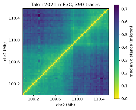
distance_map(cd, chrom) is the population median (or stat="mean") 3-D distance of every bin pair of one chromosome: per trace the Euclidean distance between its two spots, then reduced over traces with missing spots skipped (a trace that observed a bin twice contributes its last spot). It returns a DistanceMap — a dict with attribute access: matrix, count (traces observing each pair), bins (the rows), n_traces, and how it was computed.

chrom = "chr2"
dm = fea.distance_map(cd, chrom, stat="median")
print({k: dm[k] for k in ("chrom", "stat", "n_traces", "streaming", "n_passes", "n_bands")})
print("matrix", dm.matrix.shape, "| traces per pair: median", int(np.median(dm.count[np.triu_indices(60, 1)])))
dm.bins.head(3)

{'chrom': 'chr2', 'stat': 'median', 'n_traces': 390, 'streaming': False, 'n_passes': 2, 'n_bands': 1}
matrix (60, 60) | traces per pair: median 124

	bin_id	chrom	start	end
0	660	chr2	109000000	109025000
1	661	chr2	109025000	109050000
2	662	chr2	109050000	109075000

mb = dm.bins["start"].to_numpy() / 1e6
extent = [mb[0], mb[-1] + 0.025, mb[0], mb[-1] + 0.025]
fig, ax = plt.subplots(figsize=(5, 4.2))
im = ax.imshow(dm.matrix, cmap="viridis_r", origin="lower", extent=extent)
fig.colorbar(im, ax=ax, label=f"median distance ({cd.uns['xyz_unit']})")
ax.set_xlabel(f"{chrom} (Mb)"); ax.set_ylabel(f"{chrom} (Mb)")
ax.xaxis.set_major_locator(MaxNLocator(4)); ax.yaxis.set_major_locator(MaxNLocator(4))
ax.set_title(f"Takei 2021 mESC, {dm.n_traces} traces")
fig.tight_layout(); plt.show()

mean_distance_matrix(df) is the dense reference: it builds the (n_traces, n_bins, n_bins) tensor from a flat table (cd.to_dataframe()). Same definition, so the median maps are identical; distance_map never builds the tensor and therefore also runs on genome-wide data.

df = cd.get_chrom(chrom).to_dataframe()
ref, ref_bins, n_ref = fea.mean_distance_matrix(df, chrom=chrom, reduce="median")
print("median maps identical:", np.array_equal(ref, dm.matrix, equal_nan=True), "| traces:", n_ref)
ref_mean, _, _ = fea.mean_distance_matrix(df, chrom=chrom, reduce="mean")
dm_mean = fea.distance_map(cd, chrom, stat="mean")
print(f"mean maps: max |difference| = {np.nanmax(np.abs(ref_mean - dm_mean.matrix)):.1e} {cd.uns['xyz_unit']}")

median maps identical: True | traces: 390
mean maps: max |difference| = 4.4e-16 micron

Streaming over a store

On a store opened with backed=True, distance_map streams the traces in batches (iter_traces(chrom=..., columns="coords")) and computes the exact median one row band of the matrix at a time, so memory is bounded by memory_budget (default uchrom.settings.memory_budget), not by the number of traces. A deliberately small budget forces several bands; the result is the same matrix.

store = OUT / "takei2021_mesc.chromdata.zarr"
cd.write(store)
backed = ChromData.read(store, backed=True)
dm_s = fea.distance_map(backed, chrom, memory_budget="64MB")
print({k: dm_s[k] for k in ("streaming", "n_passes", "n_bands")})
print("identical to the in-memory map:", np.array_equal(dm_s.matrix, dm.matrix, equal_nan=True))

{'streaming': True, 'n_passes': 3, 'n_bands': 2}
identical to the in-memory map: True

Contact frequency, distance scaling and radius of gyration

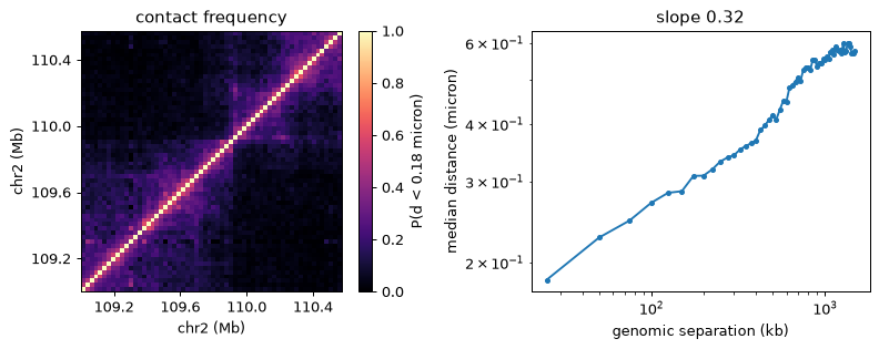
contact_frequency(df, threshold) is the fraction of traces (that observed both bins) in which two bins are closer than threshold. We use the median distance between adjacent 25-kb bins as the threshold. The decay of the median distance with genomic separation is read off the diagonals of the distance map, and radius_of_gyration(df) gives one Rg per trace.

adjacent = float(np.nanmedian(np.diag(dm.matrix, 1)))
threshold = round(adjacent, 2)
freq, _, _ = fea.contact_frequency(df, threshold, chrom=chrom)
print(f"median adjacent-bin distance {adjacent:.3f} {cd.uns['xyz_unit']} -> threshold {threshold}")
print(f"contact frequency: adjacent bins {np.nanmean(np.diag(freq, 1)):.2f}, "
      f"bins 1 Mb apart {np.nanmean(np.diag(freq, 40)):.2f}")

sep_kb = 25 * np.arange(1, 60)
med_by_sep = np.array([np.nanmedian(np.diag(dm.matrix, k)) for k in range(1, 60)])
slope = np.polyfit(np.log10(sep_kb), np.log10(med_by_sep), 1)[0]
print(f"median distance ~ separation^{slope:.2f} over 25 kb - 1.5 Mb")

fig, axes = plt.subplots(1, 2, figsize=(9, 3.6))
im = axes[0].imshow(freq, cmap="magma", origin="lower", vmin=0, vmax=1, extent=extent)
fig.colorbar(im, ax=axes[0], label=f"P(d < {threshold} {cd.uns['xyz_unit']})")
axes[0].set_xlabel(f"{chrom} (Mb)"); axes[0].set_ylabel(f"{chrom} (Mb)"); axes[0].set_title("contact frequency")
axes[0].xaxis.set_major_locator(MaxNLocator(4)); axes[0].yaxis.set_major_locator(MaxNLocator(4))
axes[1].loglog(sep_kb, med_by_sep, "o-", ms=3)
axes[1].set_xlabel("genomic separation (kb)"); axes[1].set_ylabel(f"median distance ({cd.uns['xyz_unit']})")
axes[1].set_title(f"slope {slope:.2f}")
fig.tight_layout(); plt.show()

median adjacent-bin distance 0.184 micron -> threshold 0.18
contact frequency: adjacent bins 0.49, bins 1 Mb apart 0.02
median distance ~ separation^0.32 over 25 kb - 1.5 Mb

flat = cd.to_dataframe()
rg = pd.concat({c: fea.radius_of_gyration(flat, chrom=c) for c in cd.chroms}, names=["chrom", "trace_id"])
rg_table = rg.groupby(level="chrom", sort=False).agg(["count", "median"]).rename(columns={"count": "traces", "median": "median Rg"})
print(f"{rg.notna().sum():,} traces; median Rg {rg.median():.3f} {cd.uns['xyz_unit']} "
      f"(per-locus medians {rg_table['median Rg'].min():.2f}-{rg_table['median Rg'].max():.2f})")
rg_table.sort_values("median Rg").T.round(3)

7,626 traces; median Rg 0.323 micron (per-locus medians 0.27-0.42)

chrom	chr18	chr6	chr5	chr4	chr15	chr17	chr14	chr12	chr3	chr2	chr8	chrX	chr16	chr9	chr10	chr1	chr13	chr19	chr11	chr7
traces	404.000	383.000	382.000	396.000	381.000	396.000	388.000	394.000	392.000	390.000	405.000	198.000	381.000	391.000	388.000	386.000	393.000	393.000	404.000	381.000
median Rg	0.272	0.281	0.282	0.293	0.296	0.301	0.306	0.311	0.314	0.318	0.325	0.329	0.329	0.336	0.337	0.343	0.376	0.383	0.397	0.422

2. Axis-wise variance features (what the callers test)

The ArcFISH-style callers in uchrom.strc (loops, TADs, compartments) do not test distances but the variance of the coordinate difference along each axis — imaging error differs between x/y and z, and a pair of loci that moves together has a small variance. uchrom.fea exposes the three building blocks:

• axis_variance_cube(cd, chrom) — per-axis (3, n_bins, n_bins) variance and count cubes;

• filter_normalize(cube) — drops per-trace outliers (beyond k_sigma × the distance-stratified spread) and divides by a LOWESS fit over genomic distance, so norm_var is ~1 on average at every separation;

• axis_weight(cd, chrom) — the weights of the three axes when the per-axis tests are combined (inversely proportional to each axis’s median per-trace variance).

device="auto" picks CUDA / MPS when available; we use the CPU here.

t = time.time()
cube = fea.axis_variance_cube(cd, chrom, device="cpu")
norm = fea.filter_normalize(cube, k_sigma=4.0, frac=0.1)
w = fea.axis_weight(cd, chrom, device="cpu")
print(f"{time.time() - t:.1f} s; cubes {norm['var'].shape} over {cube['n_traces']} traces")

iu = np.triu_indices(60, 1)
n_before, n_after = cube["count"][(slice(None),) + iu].sum(), norm["count"][(slice(None),) + iu].sum()
print(f"outlier observations removed: {n_before - n_after:,} of {n_before:,} ({(n_before - n_after) / n_before:.2%})")
print("axis weights x, y, z:", np.round(w, 3))
d = norm["genomic_distance"]
for a, name in enumerate("xyz"):
    e = norm["expected"][a]
    print(f"  {name}: expected variance {np.nanmedian(e[np.isclose(d, 25_000)]):.4f} at 25 kb, "
          f"{np.nanmedian(e[np.isclose(d, 1_000_000)]):.4f} at 1 Mb")

2.9 s; cubes (3, 60, 60) over 390 traces
outlier observations removed: 14,741 of 639,558 (2.30%)
axis weights x, y, z: [0.273 0.29  0.437]
  x: expected variance 0.0158 at 25 kb, 0.1366 at 1 Mb
  y: expected variance 0.0135 at 25 kb, 0.1570 at 1 Mb
  z: expected variance 0.0115 at 25 kb, 0.0596 at 1 Mb

fig, axes = plt.subplots(1, 2, figsize=(9, 3.6))
for a, name in enumerate("xyz"):
    order = np.argsort(d[iu])
    axes[0].loglog(d[iu][order] / 1e3, norm["expected"][a][iu][order], label=name)
axes[0].set_xlabel("genomic distance (kb)"); axes[0].set_ylabel("expected variance (LOWESS)")
axes[0].legend(title="axis"); axes[0].set_title("per-axis variance vs distance")
im = axes[1].imshow(np.average(norm["norm_var"], axis=0, weights=w), cmap="RdBu_r", vmin=0, vmax=2,
                    origin="lower", extent=extent)
fig.colorbar(im, ax=axes[1], label="weighted norm_var")
axes[1].set_xlabel(f"{chrom} (Mb)"); axes[1].set_ylabel(f"{chrom} (Mb)")
axes[1].xaxis.set_major_locator(MaxNLocator(4)); axes[1].yaxis.set_major_locator(MaxNLocator(4))
axes[1].set_title("normalised variance (< 1: move together)")
fig.tight_layout(); plt.show()

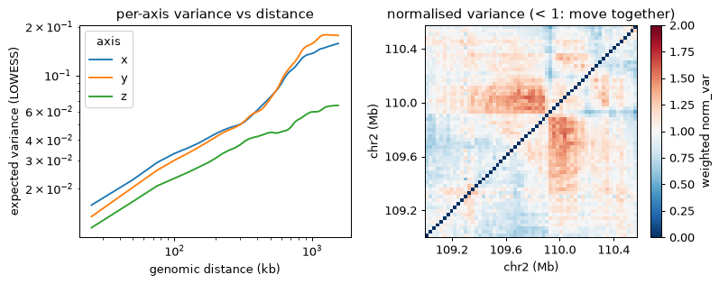
In this dataset the traces are least extended along z, so z gets the largest weight. The loop caller then F-tests norm_var of each pair against its local background; see the loop_calling and tad_calling tutorials.

3. Per-spot signals → per-locus tracks (Takei 2025 cerebellum, chr19)

The Takei 2025 store has 10.9 M spots at 100,049 genome-wide 25-kb loci and 59 immunofluorescence (IF) / repeat / RNA channels per spot (cd.spot_tracks): the intensity of a nuclear mark around that DNA locus in that cell. ds.atlas("takei2025_cerebellum") opens the store of the public U-Chrom atlas backed, over HTTP: the small tables are read at open, and range requests later fetch only chromosome 19 (a few seconds) — not the whole store.

full = ds.atlas("takei2025_cerebellum")          # backed: nothing spot-aligned is read yet
print(f"{full.n_spots:,} spots, {full.n_cells:,} cells, {full.n_bins:,} bins, "
      f"{len(full.spot_tracks.columns)} spot tracks, assembly {full.uns['genome_assembly']}")

10,912,638 spots, 1,799 cells, 100,049 bins, 62 spot tracks, assembly mm10

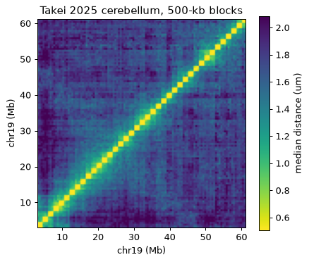
The streaming distance map is what makes such a store tractable: chr19 has 2,326 bins, and the median over its traces is computed band by band straight from the backed store. At 25 kb each trace observes only a few percent of the loci, so most pairs are seen by a handful of traces; we pool to 500 kb for display. (The default traces of this dataset can merge the two homologs — see the catalog entry — which inflates long-range distances.)

t = time.time()
dm19 = fea.distance_map(full, "chr19", memory_budget="256MB")
print(f"{time.time() - t:.1f} s: {dm19.matrix.shape[0]:,} bins, {dm19.n_traces:,} traces, "
      f"streaming={dm19.streaming}, {dm19.n_bands} bands; traces per pair: median "
      f"{np.median(dm19.count[np.triu_indices(len(dm19.matrix), 1)]):.0f}")

k = 20                                          # 20 x 25 kb = 500 kb blocks
B = len(dm19.matrix) // k * k
m19 = dm19.matrix[:B, :B].copy()
np.fill_diagonal(m19, np.nan)                   # the zero self-distances would dominate the diagonal blocks
pooled = np.nanmedian(m19.reshape(B // k, k, B // k, k).transpose(0, 2, 1, 3).reshape(B // k, B // k, -1), axis=2)
lo, hi = dm19.bins["start"].iloc[0] / 1e6, dm19.bins["start"].iloc[B - 1] / 1e6
fig, ax = plt.subplots(figsize=(5, 4.2))
im = ax.imshow(pooled, cmap="viridis_r", origin="lower", extent=[lo, hi, lo, hi],
               vmin=np.nanpercentile(pooled, 2), vmax=np.nanpercentile(pooled, 98))
fig.colorbar(im, ax=ax, label=f"median distance ({full.uns['xyz_unit']})")
ax.set_xlabel("chr19 (Mb)"); ax.set_ylabel("chr19 (Mb)"); ax.set_title("Takei 2025 cerebellum, 500-kb blocks")
fig.tight_layout(); plt.show()

6.3 s: 2,326 bins, 2,175 traces, streaming=True, 12 bands; traces per pair: median 3

Now the signals. get_chrom(..., tracks=...) reads the chromosome with just the channels we need; rebuild_bins() keeps only the loci those spots observe (2,326 chr19 bins instead of the genome’s 100,049). aggregate_tracks_by_interval averages each per-spot track over the spots of every locus (all cells, all traces) and project_interval_features_to_bins writes the result on the bin axis, cd.bin_tracks, under a prefix (with if.n_spots, the spots behind each mean).

marks = ["H3K4me3", "H3K27ac", "RNAPIISer5-P", "H3K9me3", "H3K27me3", "LaminB1"]
c19 = full.get_chrom("chr19", tracks=marks).rebuild_bins()
print(c19)

per_locus = fea.aggregate_tracks_by_interval(c19, marks, agg="mean")
print(f"{len(per_locus):,} loci; spots per locus: median {per_locus['n_spots'].median():.0f} "
      f"(min {per_locus['n_spots'].min()}, max {per_locus['n_spots'].max()})")
c19.bin_tracks = fea.project_interval_features_to_bins(c19, per_locus, prefix="if", into=c19.bin_tracks)
c19.bin_tracks.head(3).round(3)

ChromData: n_spots=178766, n_traces=2175, n_cells=1531, n_bins=2326
  spots:   ['chrom', 'start', 'end', 'trace_id', 'cell_id', 'name', 'bin_id']
  cells:   ['leiden', 'cell_type', 'x_centroid', 'y_centroid', 'z_centroid', 'nuc_volume_um3', 'doublet', 'batch'] (1531 cells)
  cellm:   {'umap': (1531, 2)}
  spot_tracks:    ['H3K9me3', 'LaminB1', 'RNAPIISer5-P', 'H3K27ac', 'H3K4me3', 'H3K27me3']
  traces:  ['dbscan_allele', 'dbscan_ldp_allele'] (2175 traces)
  uns:     ['allele_col', 'genome_assembly', 'keep_unclustered', 'source', 'voxel_xy_nm', 'voxel_z_nm', 'xyz_unit', 'zenodo_record', 'leiden_to_cell_type', 'fovs']
2,326 loci; spots per locus: median 74 (min 9, max 216)

	if.H3K4me3	if.H3K27ac	if.RNAPIISer5-P	if.H3K9me3	if.H3K27me3	if.LaminB1	if.n_spots
bin_id
0	1.667	1.205	1.287	-0.053	0.183	0.030	28
1	2.007	1.228	1.548	-0.077	0.441	-0.395	41
2	1.828	0.994	1.586	-0.059	0.373	-0.165	44

rho = c19.bin_tracks[[f"if.{m}" for m in marks]].corr(method="spearman")
rho.index = rho.columns = marks
rho.round(2)

	H3K4me3	H3K27ac	RNAPIISer5-P	H3K9me3	H3K27me3	LaminB1
H3K4me3	1.00	0.91	0.96	-0.73	0.10	-0.54
H3K27ac	0.91	1.00	0.96	-0.76	0.12	-0.39
RNAPIISer5-P	0.96	0.96	1.00	-0.77	0.15	-0.47
H3K9me3	-0.73	-0.76	-0.77	1.00	-0.06	0.32
H3K27me3	0.10	0.12	0.15	-0.06	1.00	-0.09
LaminB1	-0.54	-0.39	-0.47	0.32	-0.09	1.00

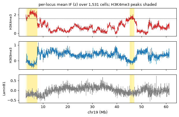
Across chr19 loci the active marks (H3K4me3, H3K27ac, initiating Pol II) rise and fall together and opposite to H3K9me3 / lamina; H3K27me3 is nearly independent of both.

aggregate_tracks_by_interval does not register what it computed; append_feature_registry_entry records your own features in the same registry the built-in writers use.

fea.append_feature_registry_entry(c19, {
    "feature_group": "spot_track_mean",
    "features": [f"if.{m}" for m in marks] + ["if.n_spots"],
    "parameters": {"aggregation": "mean", "source": "cd.spot_tracks", "chrom": "chr19"},
    "created_by": "features tutorial",
})
c19.uns["feature_registry"][-1]

{'feature_group': 'spot_track_mean',
 'features': ['if.H3K4me3',
  'if.H3K27ac',
  'if.RNAPIISer5-P',
  'if.H3K9me3',
  'if.H3K27me3',
  'if.LaminB1',
  'if.n_spots'],
 'parameters': {'aggregation': 'mean',
  'source': 'cd.spot_tracks',
  'chrom': 'chr19'},
 'created_by': 'features tutorial',
 'created_utc': '2026-10-06T22:59:15+00:00',
 'uchrom_version': '0.2.0',
 'n_features': 7}

4. Peaks of a per-locus signal

call_peaks_from_track(cd, track, method=...) aggregates a track per locus, calls peaks and writes three features per bin (peak.<name>_overlap, _count, distance_to_<name>) to cd.bin_tracks; the peak table goes to cd.results["peaks:<name>"]. Methods: "threshold" (contiguous bins above a value or quantile), "macs" (a port of MACS3 bdgpeakcall: bins at or above cutoff, merged across gaps ≤ max_gap bp, at least min_length bp) and "macs_poisson" (dynamic local-lambda Poisson test, optionally against a control_track).

IF intensities are z-scored per spot, so the cutoff is on that scale: we take the chromosome’s median locus value + 2 robust SDs (1.4826 × MAD), require two bins (50 kb) and bridge one-bin gaps. These IF “peaks” are loci that sit in an H3K4me3-rich nuclear neighbourhood, not ChIP-seq peaks.

v = per_locus["H3K4me3"]
center, spread = v.median(), 1.4826 * (v - v.median()).abs().median()
cutoff = float(center + 2 * spread)
peaks = fea.call_peaks_from_track(c19, "H3K4me3", method="macs", cutoff=cutoff,
                                  min_length=50_000, max_gap=25_000)
print(f"cutoff {cutoff:.3f}: {len(peaks)} peaks covering {(peaks['end'] - peaks['start']).sum() / 1e6:.2f} Mb "
      f"({c19.bin_tracks['peak.h3k4me3_overlap'].sum():.0f} of {c19.n_bins:,} loci)")
print("results:", list(c19.results.keys()))
peaks[["peak_id", "chrom", "start", "end", "n_bins", "score", "mean_signal", "summit"]]

cutoff 1.579: 9 peaks covering 5.60 Mb (220 of 2,326 loci)
results: ['peaks:h3k4me3', 'bin_features']

	peak_id	chrom	start	end	n_bins	score	mean_signal	summit
0	h3k4me3_1	chr19	3050000	3125000	3	2.007176	1.833974	3087500
1	h3k4me3_2	chr19	3475000	7625000	162	2.585290	2.047956	5112500
2	h3k4me3_3	chr19	45275000	45325000	2	1.699492	1.698749	45287500
3	h3k4me3_4	chr19	45375000	45425000	2	1.673454	1.669143	45412500
4	h3k4me3_5	chr19	45475000	45675000	7	1.942982	1.731808	45637500
5	h3k4me3_6	chr19	45725000	46300000	21	1.853214	1.725412	46262500
6	h3k4me3_7	chr19	46375000	46725000	11	2.030440	1.757750	46562500
7	h3k4me3_8	chr19	46875000	46950000	2	1.625147	1.623102	46937500
8	h3k4me3_9	chr19	47000000	47075000	3	1.645112	1.609127	47037500

Most peaks are a few hundred kb; one is a 4-Mb block (3.5–7.6 Mb), the gene-dense end of chr19, where the whole region sits in an H3K4me3-rich neighbourhood (see the tracks below).

The lower-level call_macs_bdgpeaks_from_signal takes any per-locus table (chrom, start, end

• a score column) — here the robust z-score of the same signal with cutoff=2, which must give the same intervals — and macs_bdgpeaks_to_narrowpeak renders the result as a narrowPeak file for a genome browser. Storing the table in cd.intervals (kind peak) lets the U-Chrom web browser draw it as an interval row.

scored = per_locus[["chrom", "start", "end"]].assign(score=(v - center) / spread)
peaks_z = fea.call_macs_bdgpeaks_from_signal(scored, signal_col="score", cutoff=2.0,
                                             min_length=50_000, max_gap=25_000, name="H3K4me3")
same = peaks_z[["start", "end"]].reset_index(drop=True).equals(peaks[["start", "end"]].reset_index(drop=True))
print("same intervals as call_peaks_from_track:", same)
narrow = OUT / "takei2025_chr19_H3K4me3.narrowPeak"
narrow.write_text(fea.macs_bdgpeaks_to_narrowpeak(peaks_z, name="H3K4me3"))
print(narrow); print("".join(narrow.read_text().splitlines(True)[:3]))

c19.intervals.add("peaks.h3k4me3", peaks, kind="peak", source_result="peaks:h3k4me3")
in_peak = c19.intervals.to_bins("peaks.h3k4me3", c19.bins, how="bool")
print("IntervalTable.to_bins agrees with peak.h3k4me3_overlap:",
      np.array_equal(in_peak.to_numpy(), c19.bin_tracks["peak.h3k4me3_overlap"].to_numpy() == 1))

same intervals as call_peaks_from_track: True
_out/takei2025_chr19_H3K4me3.narrowPeak
chr19	3050000	3125000	H3K4me3_narrowPeak1	28	.	0	0	0	37500
chr19	3475000	7625000	H3K4me3_narrowPeak2	40	.	0	0	0	1637500
chr19	45275000	45325000	H3K4me3_narrowPeak3	22	.	0	0	0	12500

IntervalTable.to_bins agrees with peak.h3k4me3_overlap: True

x = c19.bins["start"].to_numpy() / 1e6
fig, axes = plt.subplots(3, 1, figsize=(7, 4.6), sharex=True)
for ax, m, colour in zip(axes, ["H3K4me3", "H3K9me3", "LaminB1"], ["C3", "C0", "C7"]):
    ax.plot(x, c19.bin_tracks[f"if.{m}"], lw=0.6, color=colour)
    ax.set_ylabel(m, fontsize=9)
    for _, p in peaks.iterrows():
        ax.axvspan(p["start"] / 1e6, p["end"] / 1e6, color="gold", alpha=0.35, lw=0)
axes[0].axhline(cutoff, color="k", lw=0.6, ls="--")
axes[-1].set_xlabel("chr19 (Mb)")
axes[0].set_title(f"per-locus mean IF (z) over {c19.n_cells:,} cells; H3K4me3 peaks shaded", fontsize=10)
fig.tight_layout(); plt.show()

5. Annotation (GTF) and sequence (FASTA) features

add_annotation_features(cd, gtf) computes per bin: gene-body / exon / promoter (−2 kb … +0.5 kb of the TSS) overlap in bp and as a fraction, the number of genes, and the distance to the nearest TSS. It reads gene and exon rows of a GTF path or of a table from read_gtf. The UCSC mm10 RefSeq GTF has transcripts but no gene rows, so we build gene bodies by merging the overlapping transcripts of each gene (a gene name can occur at several places).

GTF = ds.fetch("mm10_refgene")                  # UCSC mm10 refGene GTF (13 MB; downloaded once)
t = time.time()
gtf = fea.read_gtf(GTF)
gtf = gtf[gtf["chrom"] == "chr19"]

tx = gtf[gtf["feature"] == "transcript"].sort_values(["gene_id", "strand", "start"])
key = tx["gene_id"] + tx["strand"]
reach = tx.groupby(key, sort=False)["end"].cummax().shift()
tx = tx.assign(locus=((key != key.shift()) | (tx["start"] > reach)).cumsum())
genes = (tx.groupby("locus")
           .agg(chrom=("chrom", "first"), start=("start", "min"), end=("end", "max"),
                strand=("strand", "first"), gene_id=("gene_id", "first"))
           .assign(feature="gene"))
annotation = pd.concat([genes, gtf[gtf["feature"] == "exon"]], ignore_index=True)
print(f"{len(genes)} chr19 genes, {(gtf['feature'] == 'exon').sum():,} exons")

ann = fea.add_annotation_features(c19, annotation)
print(f"{time.time() - t:.1f} s"); ann.drop(columns=["chrom", "start", "end"]).describe().loc[["mean", "50%", "max"]].round(3)

815 chr19 genes, 14,101 exons

3.3 s

	gene_body_overlap_bp	gene_body_overlap_fraction	gene_count	exon_overlap_bp	exon_overlap_fraction	promoter_overlap_bp	promoter_overlap_fraction	nearest_tss_distance
mean	12368.102	0.495	0.858	955.059	0.038	824.108	0.033	96587.617
50%	12860.000	0.514	1.000	115.000	0.005	0.000	0.000	24824.000
max	25000.000	1.000	8.000	20480.000	0.819	12836.000	0.513	1218976.000

add_sequence_features(cd, fasta) computes GC fraction, CpG density, N fraction and G-quadruplex motif counts per bin from a (gzipped) FASTA whose record names are the chromosome names. It needs only the chromosomes of the bins: the UCSC mm10 chr19.fa.gz (19 MB, ds.fetch("mm10_chr19")) suffices here.

FASTA = ds.fetch("mm10_chr19")                  # UCSC mm10 chr19 sequence (19 MB; downloaded once)
t = time.time()
seq = fea.add_sequence_features(c19, FASTA)
print(f"{time.time() - t:.1f} s"); seq.drop(columns=["chrom", "start", "end"]).describe().loc[["mean", "50%", "max"]].round(4)

1.6 s

	gc_fraction	cpg_density	n_fraction	g4_motif_count	g4_motif_density
mean	0.4273	0.0096	0.0004	11.0387	0.0004
50%	0.4207	0.0087	0.0000	8.0000	0.0003
max	0.5583	0.0298	0.5446	143.0000	0.0057

Do the imaging signals agree with the genome?

A check on real data: loci in H3K4me3 peaks should be gene- and promoter-rich and GC-rich, and the active marks should correlate with GC content and promoter density, the repressive ones against them.

bt = c19.bin_tracks
inside = bt["peak.h3k4me3_overlap"] == 1
summary = pd.DataFrame({
    "in H3K4me3 peaks": [inside.sum(), (bt["gtf.promoter_overlap_bp"] > 0)[inside].mean(),
                          bt["gtf.gene_count"][inside].mean(), bt["seq.gc_fraction"][inside].median()],
    "other loci": [(~inside).sum(), (bt["gtf.promoter_overlap_bp"] > 0)[~inside].mean(),
                   bt["gtf.gene_count"][~inside].mean(), bt["seq.gc_fraction"][~inside].median()],
}, index=["loci", "fraction with a promoter", "genes per locus", "median GC"])
display(summary.round(3))

rows = {}
for m in marks:
    rows[m] = {f: spearmanr(bt[f"if.{m}"], bt[f], nan_policy="omit")[0]
               for f in ["seq.gc_fraction", "seq.cpg_density", "gtf.promoter_overlap_fraction", "gtf.nearest_tss_distance"]}
pd.DataFrame(rows).T.round(2)

	in H3K4me3 peaks	other loci
loci	220.000	2106.000
fraction with a promoter	0.609	0.243
genes per locus	1.691	0.771
median GC	0.485	0.417

	seq.gc_fraction	seq.cpg_density	gtf.promoter_overlap_fraction	gtf.nearest_tss_distance
H3K4me3	0.68	0.61	0.31	-0.46
H3K27ac	0.67	0.62	0.23	-0.36
RNAPIISer5-P	0.70	0.64	0.27	-0.40
H3K9me3	-0.64	-0.59	-0.22	0.33
H3K27me3	0.16	0.16	-0.17	0.15
LaminB1	-0.34	-0.25	-0.21	0.25

6. The feature registry and persistence

Every writer appended a provenance record to cd.uns["feature_registry"]: the feature group, the columns it wrote, the parameters, the source file, the U-Chrom version and a timestamp. The interval tables behind the bin features are in cd.results["bin_features"] (one row per locus).

reg = pd.DataFrame(c19.uns["feature_registry"])
display(reg[["feature_group", "created_by", "n_features", "result_key", "uchrom_version"]])
peaks_record = next(r for r in c19.uns["feature_registry"] if r["feature_group"] == "peaks")
print({k: peaks_record["parameters"][k] for k in ("method", "aggregation", "cutoff", "min_length", "max_gap")})

	feature_group	created_by	n_features	result_key	uchrom_version
0	spot_track_mean	features tutorial	7	NaN	0.2.0
1	peaks	uchrom.fea.peaks	3	bin_features	0.2.0
2	annotation	uchrom.fea.annotation	8	bin_features	0.2.0
3	sequence	uchrom.fea.sequence	5	bin_features	0.2.0

{'method': 'macs_bdgpeakcall', 'aggregation': 'mean', 'cutoff': 1.579222762762184, 'min_length': 50000, 'max_gap': 25000}

path = OUT / "takei2025_chr19_features.chromdata.zarr"
c19.write(path)
back = ChromData.read(path)
print(path)
print("bin_tracks:", back.bin_tracks.shape, "| results:", list(back.results.keys()),
      "| intervals:", list(back.intervals), "| registry entries:", len(back.uns["feature_registry"]))
print("bin_tracks round trip equal:", back.bin_tracks.equals(c19.bin_tracks))

_out/takei2025_chr19_features.chromdata.zarr
bin_tracks: (2326, 23) | results: ['peaks:h3k4me3', 'bin_features'] | intervals: ['peaks.h3k4me3'] | registry entries: 4
bin_tracks round trip equal: True

Next steps

• loop_calling, tad_calling, compartment — the callers built on the axis-wise variance features of section 2.

• plotting_and_browser — the uchrom.pl figures and the web browser, which shows bin_tracks, spot_tracks and cd.intervals (e.g. the store written above) as genome tracks.

• import_seqfish_multiomics — more of the Takei 2025 cerebellum data (cell types, embeddings).