Concepts

Three kinds of 3-D genome data

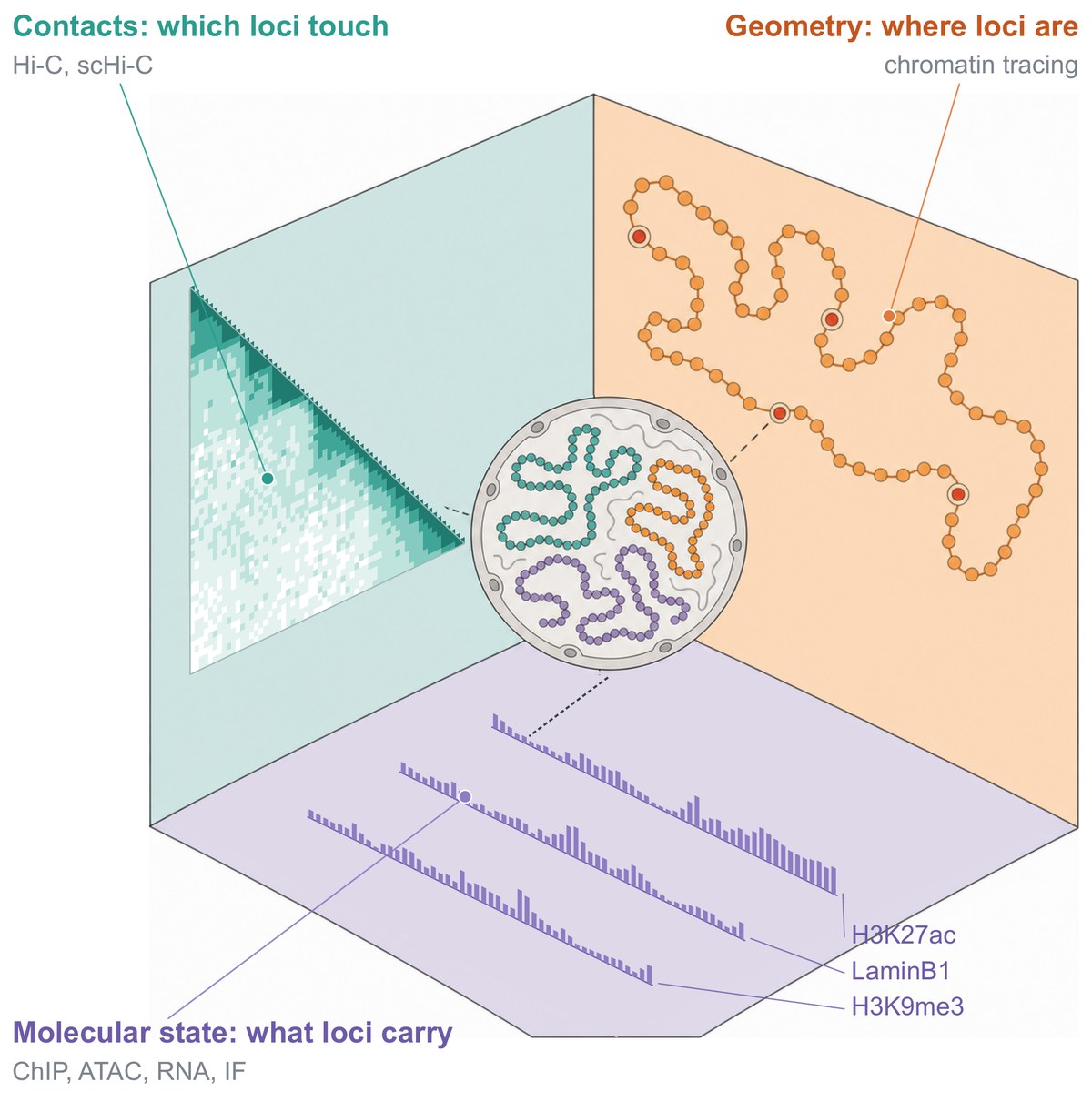
Each assay captures one facet of 3-D genome organisation: contacts (Hi-C, single-cell Hi-C: which loci touch), geometry (chromatin tracing: where loci are) and molecular state (ChIP, ATAC, RNA, immunofluorescence: what loci carry). The contact map is scHiCAR of the mouse motor cortex, the tracks are chromatin marks of one cerebellar cell measured by DNA seqFISH+. From Fig. 1a of the U-Chrom paper; the illustration is AI-generated and edited by the authors and, apart from the contact map and the signal tracks, conceptual.

Sequencing and imaging measure different things, at different resolutions, in different numbers of cells — and each field has its own formats and tools. What they share is the genome: every measurement is about loci.

One shared index, not a joint model

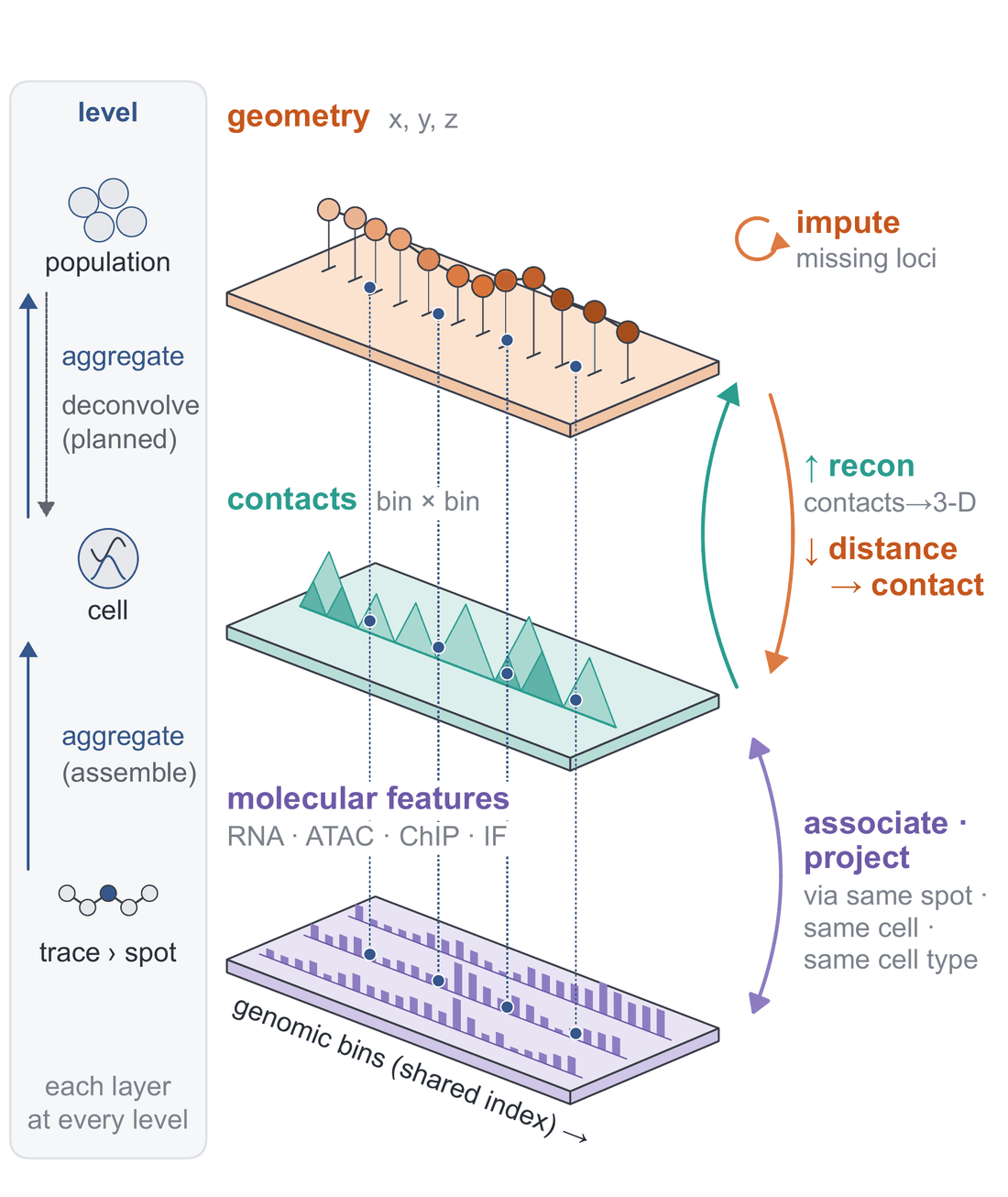
ChromData keeps each modality as its own layer — geometry (x, y, z), contacts (bin × bin maps, linked when large), molecular features — and indexes all of them by the same genomic bins (dashed lines). Left, any layer can be held per population, per cell or per trace › spot; aggregation moves data up a level. Right, operations within and between layers: imputation, reconstruction of 3-D from contacts, conversion of distances into contact frequencies; molecular features are projected onto structures through a shared spot, cell or cell type. From Fig. 1b of the U-Chrom paper.

Nothing is forced into one matrix: a chromatin-tracing experiment fills the geometry layer, a single-cell Hi-C experiment the contact layer (and, after reconstruction, geometry too), a seqFISH+ multi-omics experiment geometry and molecular features in the same cells. The shared bins are what lets one analysis read another’s output.

The central table is the one every 3-D measurement ends in — a locus and where it is:

chrom	start	end	x	y	z
chr3	34,600,000	34,625,000	1.82	0.44	−0.91
chr3	34,625,000	34,650,000	1.79	0.47	−0.88

Chromatin tracing and DNA seqFISH+ measure the positions directly; Hi-C measures contacts, from which reconstruction computes them. Everything downstream — distances, structures, features, the browser — works on this table, whatever produced it.

Cells, traces, spots — and bins

• A spot is one locus observed in 3-D: a row of the table.

• A trace is an ordered chain of spots along one chromatin fibre — one copy of a chromosome region (two per diploid cell, or one per haplotype after phasing).

• A cell holds traces (and, for sequencing data, contact maps and other modalities).

• A bin is a locus of the locus axis shared by all cells: chrom, start, end. Every spot points at one bin (spots.bin_id), so signals that belong to a locus (bulk ATAC, GC content, a compartment score) are stored once per bin, not once per spot.

ChromData

ChromData (package chromdata) holds all of it, the way AnnData holds a single-cell matrix:

ChromData
├── bins         loci (n_bins): chrom, start, end, [name, resolution]
├── bin_tracks   per-locus signals (n_bins)
├── binm         per-locus multi-dimensional arrays
├── intervals    typed tables of structures: TADs, loops, peaks, segments
├── coords       (n_spots, 3) x, y, z
├── spots        per spot: bin_id, trace_id, [cell_id]   (chrom / start / end derived from bins)
├── spot_tracks  per-spot signals (IF intensity, RNA z-scores, ...)
├── layers       alternative coordinates (n_spots, 3): imputed, models of an ensemble, ...
├── cells        per cell: type, position, counts, ...
├── cellm        per-cell multi-dimensional arrays: embeddings, UMAP, ...
├── traces       per trace
├── cell_shapes  cell outlines (GeoParquet)
├── points       non-genomic 3-D points: RNA spots, IF puncta
├── results      analysis outputs, each with its provenance (function, parameters, version, time)
└── uns          metadata: genome assembly, units, linked files, ...

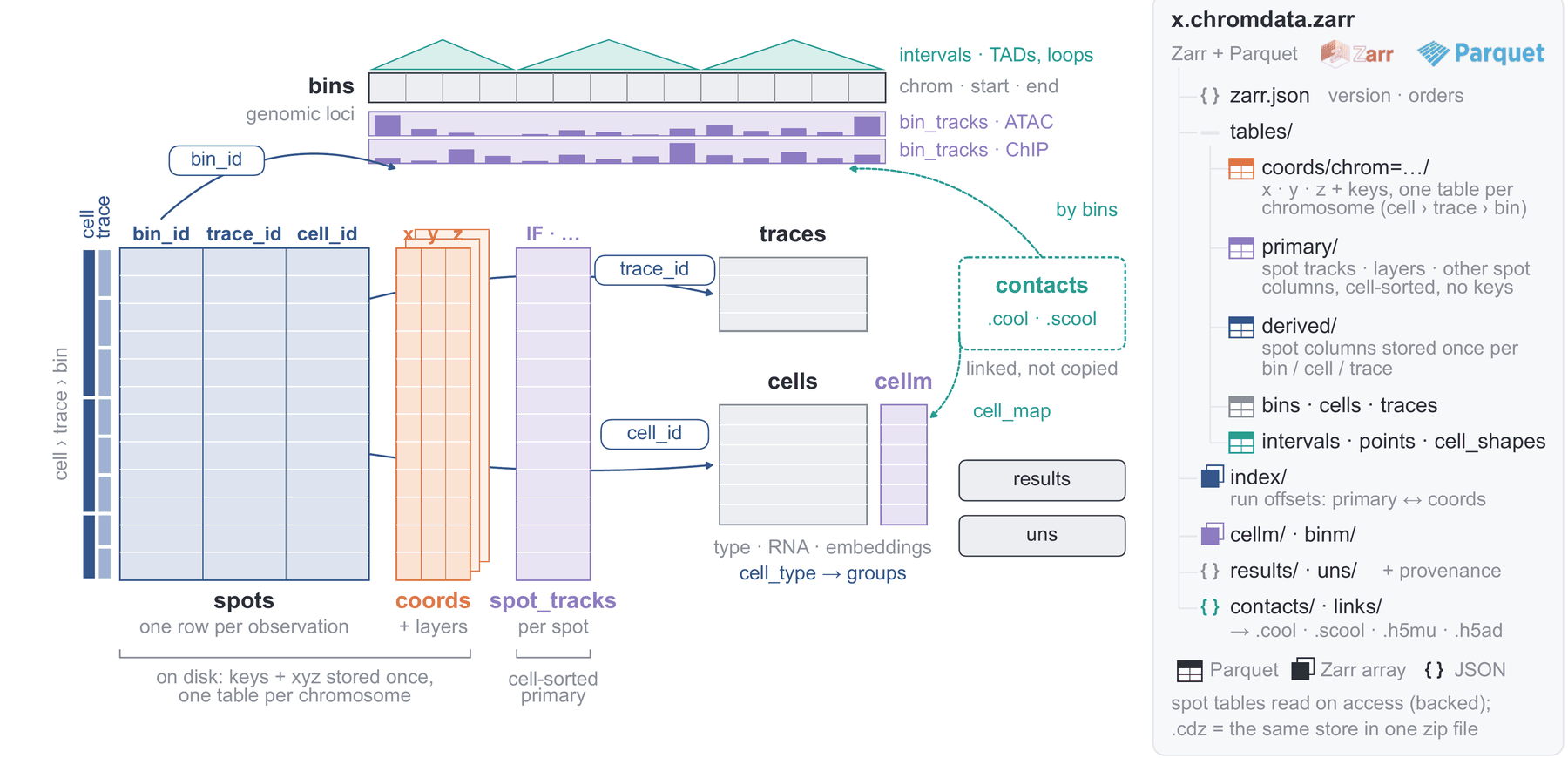
The tables of a ChromData and how they are joined: spots (one row per observation) point at the shared locus axis (bins) and at traces and cells through keys; coordinates and per-spot tracks are row-aligned with the spots; contact maps are linked, not copied. Right, the layout of a .chromdata.zarr store (Parquet tables, Zarr arrays, JSON attributes). From Fig. 2a of the U-Chrom paper.

All spots of all cells are stored flat; cd.get_cell(id), cd.get_trace(id) and cd.get_chrom(name) return the part you need as a new ChromData. Pairwise distance matrices are never stored — cd.compute_distances(trace_id=...) computes one when needed.

Linked and embedded modalities

Single-cell Hi-C contact maps (.scool), pseudo-bulk maps (.cool / .mcool), RNA or ATAC matrices (.h5ad, .h5mu), SpatialData stores and section images stay in their own files: a ChromData records links to them with the mapping between their cells and its cells (cd.link_scool, cd.link_cool, cd.link_anndata, cd.link_mudata, cd.link_spatialdata). To share a dataset as one self-contained store, the linked files are embedded into it (python -m chromdata.embedded STORE): contact maps partitioned by chromosome and sharded for range reads, AnnData as Zarr.

The store: .chromdata.zarr

cd.write("x.chromdata.zarr") writes a Zarr v3 group with Parquet tables (.cdz is the same tree in one zip file). Coordinates are partitioned by chromosome and sorted by cell; other per-spot columns sit in cell-sorted tables; an index maps cells, traces and chromosomes to row ranges. So a store opens backed — ChromData.read(path, backed=True) reads the small tables and the index, and a cell, a trace or a chromosome is read when asked for — on a laptop, on a cluster, or over HTTP from object storage (that is how the data atlas works). Large data are written by streaming (ChromData.writer) and analysed chunk by chunk (cd.iter_cells()), within a memory budget (uchrom.settings.memory_budget). The layout is specified in the format specification.

Analyses

Analysis functions follow one calling convention:

result = fn(cd, *, chrom=None, params=..., device="auto", key_added="<what>.<method>", copy=False)

chrom=None runs every chromosome; the result is returned and stored in cd.results[key_added] (structures also in cd.intervals, per-locus values in cd.bin_tracks) together with the function, its parameters and the U-Chrom version, so a store remembers how its results were made. uchrom.tl and uchrom.pp give short names: uc.tl.call_tads(cd), uc.tl.call_loops(cd), uc.tl.call_compartments(cd), uc.tl.reconstruct_sc(contacts), uc.pp.impute(cd).

The ecosystem

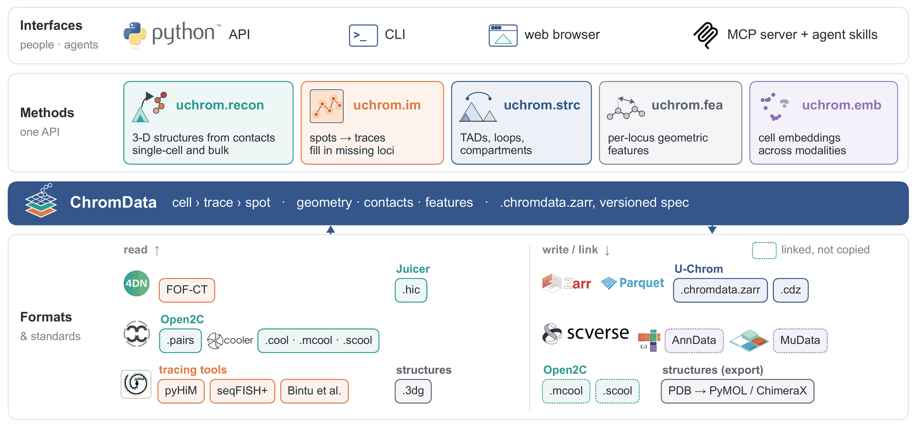
Community formats are read, or linked without copying (dashed boxes); a ChromData is stored as a .chromdata.zarr store (.cdz: the same store in one zip file); structures are exported as PDB. The analysis modules — reconstruction, imaging-side processing, structure calling, geometric features, cell embeddings — share one API, reached from Python, the command line, the web browser and agents. From Fig. 1c of the U-Chrom paper (logos are trademarks of their owners, used for identification only).

Where things live

Your data	Chapter
chromatin tracing (FOF-CT, PyHiM, raw detections)	Chromatin tracing
DNA seqFISH+ with chromatin marks and RNA	Imaging multi-omics
single-cell Hi-C, its multi-omics variants, spatial Hi-C	Single-cell and spatial Hi-C
bulk Hi-C (alone, or with tracing of the same cells)	Bulk Hi-C

You want to — for any data	Chapter
hold, subset, save, share, link	Data model & storage (chromdata)
call loops, TADs, domains, compartments	Structure calling (uchrom.strc)
compute per-locus features	Per-locus features (uchrom.fea)
compare cells	Cells & embeddings (uchrom.emb)
look at it	Visualisation (uchrom-browser, uchrom.pl)
read or write a file format	File formats (uchrom.io)